I decided to show how do a simple budget on Excel because every time I get into the swing of using Excel for school I tend to use it more in my personal life. When I started to do my Excel project my mom decided to come to me and complain about my dad who wanted to drive to Yosemite instead of taking a plane! So, since my mother is not very computer savvy and I am the one always looking for prices on tickets anyways, I decided to do a little bit more research with prices and make a budget for my dad to see and be able to play with to see what option he liked best.
So, lets start with our very own budget.
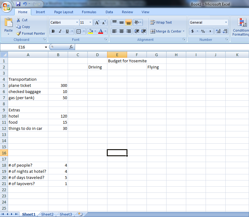
First, you need to open Excel and start on a blank work sheet.

Then type a simple title (Budget for Yosemite) and subtitle (Driving vs. Flying).
And start breaking up different expenses into categories.

Now do your own research in finding prices, the ones here are just for show, and type them in the next column to the right after the category.
Also, in the corner of my budget I put small facts, i.e. how many people are traveling [4], how many nights in the hotel [4], ext. to help me in the next step.
Next are the formulas. The ones we will be filling in right now are all going to be multiplication (*). When making a function you must start with an equal sign (=). So, for the first function in cell G5 we need to multiply the price of one plane ticket (in cell B5) with the number of people going in the trip (cell B17) which should look like =B5*B17 once that is in correctly press enter and Excel will calculate it and the answer will be in the cell. Now, just go through and multiple correctly with every cell.

After you have calculated the per price by how many days or people, we can move on to the total of both trips. You will just need to add two more categories (TOTAL and Difference) since I forgot to mention it in the beginning.
Functions. The heart and soul of Microsoft Excel. Functions are a little tricky to get use to but with a simple budget like this we will be just using the basics. With functions you still start out with and equal sign but you now will be using words to show what you want to do with your data. We need to figure out the total of each trip separately. Lets use the SUM function. Go to cell D14 and type in "=SUM(", then highlight the cells you want it to calculate, from D5 to D2, close parentheses and hit enter. Do the same for column G.
Next to "Difference" find a cell in between the two totals and find the difference. Use the steps that we used from the formulas with the subtraction sign being a hyphen (-).

Now that all the calculations are done you can add bold the categories and title, color to the difference, and make some boarders so it is easier to read. To bold you just click the cell and go up to the font section in the Home ribbon and click the bold character. To color text you click the cell you want and go to the same section as the bold but click the A with a line of color underneath it. To create boarders you start at the beginning or top of what you want and drag to the end or bottom. Again, go to the font section in the Home ribbon and click the box that has broken dots and a solid line and pick your desired boarder.

With this simple and easy to read budget plan you can easily go and change the price of a ticket or the number of people joining you on the trip and Excel will do the calculations for you. It is a quick and easy way to determine how much you need to save and can be reused over and over again.
All images were made by Lauren Robert with Microsoft's Excel.